
The normal distribution or Gaussian distribution is the probability distribution in a continuous variable, in which the probability density function is described by an exponential function of quadratic and negative argument, which gives rise to a bell shape.
The name of normal distribution comes from the fact that this distribution is the one that applies to the greatest number of situations where some continuous random variable is involved in a given group or population..
Examples where the normal distribution is applied are: the height of men or women, variations in the measure of some physical magnitude or in measurable psychological or sociological traits such as the intellectual quotient or the consumption habits of a certain product.
On the other hand, it is called a Gaussian distribution or Gaussian bell, because it is this German mathematical genius who is credited with his discovery for the use he gave it for the description of the statistical error of astronomical measurements back in the year 1800..
However, it is stated that this statistical distribution was previously published by another great mathematician of French origin, such as Abraham de Moivre, back in the year 1733.
Article index
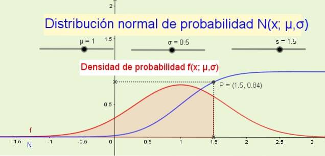
To the normal distribution function in the continuous variable x, with parameters μ Y σ it is denoted by:
N (x; μ, σ)
and it is explicitly written like this:
N (x; μ, σ) = ∫-∞x f (s; μ, σ) ds
where f (u; μ, σ) is the probability density function:
f (s; μ, σ) = (1 / (σ√ (2π)) Exp (- stwo/ (2σtwo))
The constant that multiplies the exponential function in the probability density function is called the normalization constant, and it has been chosen in such a way that:
N (+ ∞, μ, σ) = 1
The previous expression ensures that the probability that the random variable x is between -∞ and + ∞ is 1, that is, 100% probability.
Parameter μ is the arithmetic mean of the continuous random variable x y σ the standard deviation or square root of the variance of that same variable. In the event that μ = 0 Y σ = 1 then we have the standard normal distribution or typical normal distribution:
N (x; μ = 0, σ = 1)
1- If a random statistical variable follows a normal probability density distribution f (s; μ, σ), most of the data is clustered around mean value μ and are scattered around it such that little more than ⅔ of the data is between μ - σ Y μ + σ.
2- The standard deviation σ it is always positive.
3- The form of the density function F resembles that of a bell, which is why this function is often called a Gaussian bell or Gaussian function.
4- In a Gaussian distribution the mean, the median and the mode coincide.
5- The inflection points of the probability density function are located precisely at μ - σ Y μ + σ.
6- The function f is symmetric with respect to an axis that passes through its mean value μ y has asymptotically zero for x ⟶ + ∞ and x ⟶ -∞.
7- The higher the value of σ greater dispersion, noise or distance of the data around the mean value. That is to say greater σ the bell shape is more open. Instead σ small indicates that the dice are tight to the middle and the shape of the bell is more closed or pointed.
8- The distribution function N (x; μ, σ) indicates the probability that the random variable is less than or equal to x. For example, in Figure 1 (above) the probability P that the variable x is less than or equal to 1.5 is 84% and corresponds to the area under the probability density function f (x; μ, σ) from -∞ to x.
9- If the data follow a normal distribution, then 68.26% of these are between μ - σ Y μ + σ.
10- 95.44% of the data that follow a normal distribution are found between μ - 2σ Y μ + 2σ.
11- 99.74% of the data that follow a normal distribution are between μ - 3σ Y μ + 3σ.
12- If a random variable x follow a distribution N (x; μ, σ), then the variable
z = (x - μ) / σ follows the standard normal distribution N (z, 0.1).
The change of the variable x to z It is called standardization or typing and is very useful when applying the tables of the standard distribution to data that follow a non-standard normal distribution.
To apply the normal distribution it is necessary to go through the calculation of the integral of the probability density, which from the analytical point of view is not easy and there is not always a computer program that allows its numerical calculation. For this purpose, the tables of normalized or standardized values are used, which is nothing more than the normal distribution in the case μ = 0 and σ = 1.
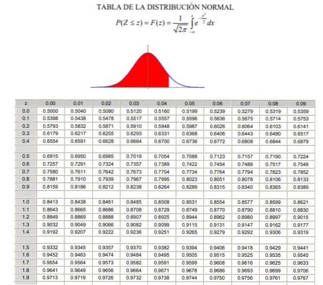
It should be noted that these tables do not include negative values. However, using the symmetry properties of the Gaussian probability density function the corresponding values can be obtained. In the resolved exercise shown below, the use of the table in these cases is indicated.
Suppose you have a set of random data x that follow a normal distribution of mean 10 and standard deviation 2. You are asked to find the probability that:
a) The random variable x is less than or equal to 8.
b) Is less than or equal to 10.
c) That the variable x is below 12.
d) The probability that a value x is between 8 and 12.
Solution:
a) To answer the first question you simply have to calculate:
N (x; μ, σ)
With x = 8, μ = 10 Y σ = 2. We realize that it is an integral that does not have an analytical solution in elementary functions, but the solution is expressed as a function of the error function erf (x).
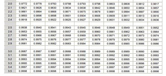
On the other hand, there is the possibility of solving the integral in numerical form, which is what many calculators, spreadsheets and computer programs such as GeoGebra do. The following figure shows the numerical solution corresponding to the first case:
and the answer is that the probability that x is below 8 is:
P (x ≤ 8) = N (x = 8; μ = 10, σ = 2) = 0.1587
b) In this case, we try to find the probability that the random variable x is below the mean, which in this case is worth 10. The answer does not require any calculation, since we know that half of the data are below average and the other half above average. Therefore, the answer is:
P (x ≤ 10) = N (x = 10; μ = 10, σ = 2) = 0.5
c) To answer this question you have to calculate N (x = 12; μ = 10, σ = 2), This can be done with a calculator that has statistical functions or through software such as GeoGebra:
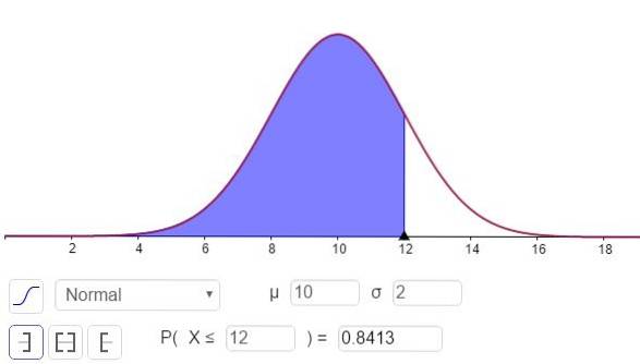
The answer to part c can be seen in figure 3 and is:
P (x ≤ 12) = N (x = 12; μ = 10, σ = 2) = 0.8413.
d) To find the probability that the random variable x is between 8 and 12 we can use the results of parts a and c as follows:
P (8 ≤ x ≤ 12) = P (x ≤ 12) - P (x ≤ 8) = 0.8413 - 0.1587 = 0.6826 = 68.26%.
The average price of a company's stock is $ 25 with a standard deviation of $ 4. Determine the probability that:
a) An action has a cost less than $ 20.
b) That has a cost greater than $ 30.
c) The price is between $ 20 and $ 30.
Use Standard Normal Distribution Tables to Find Answers.
Solution:
To be able to make use of the tables, it is necessary to pass to the normalized or typed z variable:
$ 20 in the normalized variable equals z = ($ 20 - $ 25) / $ 4 = -5/4 = -1.25 and
$ 30 in the normalized variable equals z = ($ 30 - $ 25) / $ 4 = +5/4 = +1.25.
a) $ 20 equals -1.25 in the normalized variable, but the table does not have negative values, so we place the value +1.25 which yields the value of 0.8944.
If 0.5 is subtracted from this value, the result will be the area between 0 and 1.25 which, by the way, is identical (by symmetry) to the area between -1.25 and 0. The result of the subtraction is 0.8944 - 0.5 = 0.3944 which is the area between -1.25 and 0.
But the area from -∞ to -1.25 is of interest, which will be 0.5 - 0.3944 = 0.1056. It is therefore concluded that the probability that a stock is below $ 20 is 10.56%.
b) $ 30 in the typed variable z is 1.25. For this value, the number 0.8944 appears in the table, which corresponds to the area from -∞ to +1.25. The area between +1.25 and + ∞ is (1 - 0.8944) = 0.1056. That is, the probability that a share costs more than $ 30 is 10.56%.
c) The probability that an action has a cost between $ 20 and $ 30 will be calculated as follows:
100% -10.56% - 10.56% = 78.88%


Yet No Comments