The standard error of estimate measures the deviation in a sample population value. That is, the standard error of estimation measures the possible variations of the sample mean with respect to the true value of the population mean..
For example, if you want to know the average age of the population of a country (population mean), you take a small group of inhabitants, whom we will call a “sample”. From it, the average age (sample mean) is extracted and it is assumed that the population has that average age with a standard error of estimation that varies more or less.
It should be noted that it is important not to confuse the standard deviation with the standard error and with the standard error of estimation:
1- The standard deviation is a measure of the dispersion of the data; that is, it is a measure of the variability of the population.
2- The standard error is a measure of the variability of the sample, calculated based on the standard deviation of the population.
3- The standard error of estimation is a measure of the error that is committed when taking the sample mean as an estimate of the population mean.
Article index
The standard error of estimation can be calculated for all measurements that are obtained in the samples (for example, standard error of estimation of the mean or standard error of estimation of the standard deviation) and measures the error that is made when estimating the true population measure from its sample value
From the standard error of estimation, the confidence interval of the corresponding measure is constructed.
The general structure of a formula for the standard error of estimation is as follows:
Standard error of estimation = ± Confidence coefficient * Standard error
Confidence coefficient = limit value of a sample statistic or sampling distribution (normal or Gaussian bell, Student's t, among others) for a given probability interval.
Standard error = standard deviation of the population divided by the square root of the sample size.
The confidence coefficient indicates the number of standard errors that you are willing to add and subtract to the measure to have a certain level of confidence in the results..
Suppose you are trying to estimate the proportion of people in the population who have a behavior A, and you want to have 95% confidence in your results..
A sample of n people is taken and the sample proportion p and its complement q are determined.
Standard error of estimate (SEE) = ± Confidence coefficient * Standard error
Confidence coefficient = z = 1.96.
Standard error = the square root of the ratio between the product of the sample proportion and its complement and the sample size n.
From the standard error of estimation, the interval in which the population proportion is expected to be found or the sample proportion of other samples that can be formed from that population is established, with a 95% confidence level:
p - EEE ≤ Population proportion ≤ p + EEE
1- Suppose you are trying to estimate the proportion of people in the population who have a preference for an enriched milk formula, and you want to have 95% confidence in your results..
A sample of 800 people is taken and it is determined that 560 people in the sample have a preference for the fortified milk formula. Determine an interval in which the population proportion and the proportion of other samples that can be taken from the population can be expected to be found, with 95% confidence
a) Let's calculate the sample proportion p and its complement:
p = 560/800 = 0.70
q = 1 - p = 1 - 0.70 = 0.30
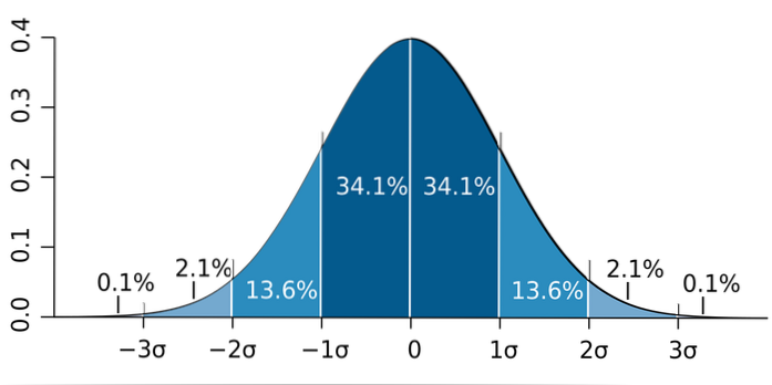
b) It is known that the proportion approximates a normal distribution to large samples (greater than 30). Then, the so-called rule 68 - 95 - 99.7 is applied and we have to:
Confidence coefficient = z = 1.96
Standard error = √ (p * q / n)
Standard error of estimate (SEE) = ± (1.96) * √ (0.70) * (0.30) / 800) = ± 0.0318
c) From the standard error of estimation, the interval in which the population proportion is expected to be found with a 95% confidence level is established:
0.70 - 0.0318 ≤ Population proportion ≤ 0.70 + 0.0318
0.6682 ≤ Population proportion ≤ 0.7318
The 70% sample proportion can be expected to change by up to 3.18 percentage points if you take a different sample of 800 individuals or that the actual population proportion is between 70 - 3.18 = 66.82% and 70 + 3.18 = 73.18%.
2- We will take from Spiegel and Stephens, 2008, the following case study:
A random sample of 50 grades was taken from the total mathematics grades of the first-year students of a university, in which the mean found was 75 points and the standard deviation, 10 points. What are the 95% confidence limits for estimating the mean college math grades??
a) Let's calculate the standard error of estimation:
95% confidence coefficient = z = 1.96
Standard error = s / √n
Standard error of estimate (SEE) = ± (1.96) * (10√50) = ± 2.7718
b) From the standard error of estimation, the interval in which the population mean or the mean of another sample of size 50 is expected to be found, with a 95% confidence level is established:
50 - 2.7718 ≤ Population average ≤ 50 + 2.7718
47.2282 ≤ Population average ≤ 52.7718
c) The sample mean can be expected to change by as much as 2.7718 points if a different sample of 50 grades is taken or that the actual mean math grades of the university population is between 47.2282 points and 52.7718 points.


Yet No Comments