Injective function what it is, what it is for and examples

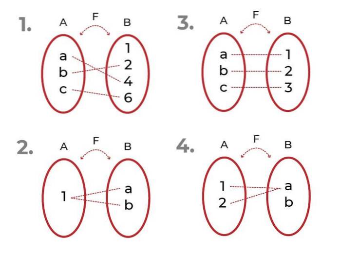
A injective function is any relationship of elements of the domain with a single element of the codomain. Also known as function one by one ( eleven ), are part of the classification of functions with respect to the way in which their elements are related.

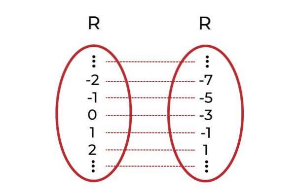
An element of the codomain can only be the image of a single element of the domain, in this way the values ​​of the dependent variable cannot be repeated.

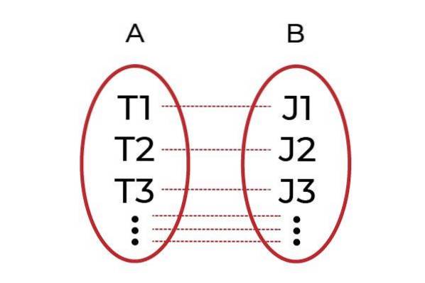
A clear example would be grouping men with jobs in group A, and in group B all the bosses. The function F It will be the one that associates each worker with his boss. If each worker is associated with a different boss through F, then F  will be a injective function.

To consider injective to a function the following must be fulfilled:

∀ x₁  ≠ x_two   ⇒ F (x₁ ) ≠ F (x_two )

This is the algebraic way of saying For all x₁ different from x_two you have an F (x₁ ) different from F (x_two ).

Article index

• 1 What are injection functions for?
  • 1.1 Function conditioning
• 2 Examples of injection functions with solved exercises
  • 2.1 Example 1
  • 2.2 Example 2
  • 2.3 Example 3
  • 2.4 Example 4
  • 2.5 Example 5
  • 2.6 Example 6
  • 2.7 Example 7
• 3 Exercises proposed for class / home
• 4 References

What are injective functions for?

Injectivity is a property of continuous functions, since they ensure the assignment of images for each element of the domain, an essential aspect in the continuity of a function..

When drawing a line parallel to the axis X on the graph of an injective function, the graph should only be touched at a single point, regardless of the height or magnitude of Y the line is drawn. This is the graphical way to test the injectivity of a function.

Another way to test if a function is injective, is solving for the independent variable X in terms of the dependent variable Y. Then it must be verified if the domain of this new expression contains the real numbers, at the same time as for each value of Y there is a single value of X.

The functions or order relations obey, among other ways, the notation F: D_F→C_F

What is read F running from D_F up to C_F

Where the function F relate the sets Domain Y Codomain. Also known as the starting set and the arrival set.

The Dominion D_F  contains the allowed values ​​for the independent variable. The codomain C_F  It is made up of all the values ​​available to the dependent variable. The elements of C_F related to D_F  are known as Function range (R_F ).

Function conditioning

Sometimes a function that is not injective can be subjected to certain conditions. These new conditions can make it a injective function. All kinds of modifications to the domain and codomain of the function are valid, where the objective is to fulfill the properties of injectivity in the corresponding relation.

Examples of injection functions with solved exercises

Example 1

Let the function F: R → R defined by the line F (x) = 2x - 3

A: [All real numbers]

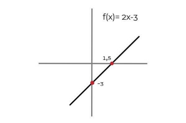
It is observed that for every value of the domain there is an image in the codomain. This image is unique which makes F an injective function. This applies to all linear functions (Functions whose greatest degree of the variable is one).

Example 2

Let the function F: R → R defined by F (x) = x^two +1

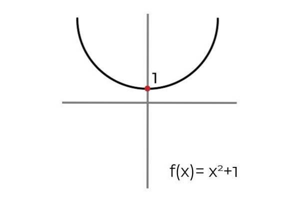
When drawing a horizontal line, it is observed that the graph is found on more than one occasion. Because of this the function F not injective as long as defined  R → R

We proceed to condition the domain of the function:

                                               F: R⁺ OR 0 → R

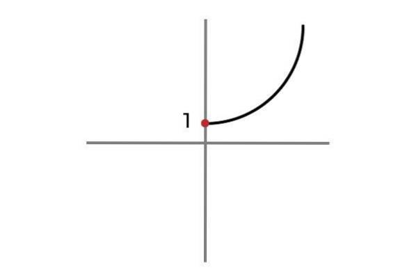
Now the independent variable does not take negative values, in this way repeating results is avoided and the function F: R⁺ OR 0 → R defined by F (x) = x^two + 1 is injective.

Another homologous solution would be to limit the domain to the left, that is, to restrict the function to only take negative and zero values.

We proceed to condition the domain of the function

                                               F: R^- OR 0 → R

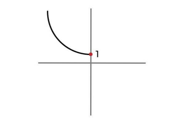
Now the independent variable does not take negative values, in this way repeating results is avoided and the function F: R^- OR 0 → R defined by F (x) = x^two + 1 is injective.

Trigonometric functions have wave-like behaviors, where it is very common to find repetitions of values ​​in the dependent variable. Through specific conditioning, based on prior knowledge of these functions, we can narrow the domain to meet the conditions of injectivity.

Example 3

Let the function F: [ -π / 2, π / 2 ] → R defined by F (x) = Cos (x)

In the interval [ -π / 2 → π / 2 ] the cosine function varies its results between zero and one.

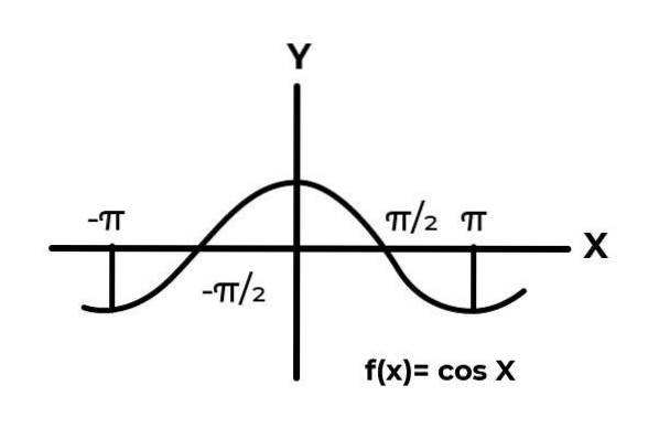
As can be seen in the graph. Start from scratch in x = -π / 2 then reaching a maximum at zero. It is after x = 0 that the values ​​begin to repeat, until they return to zero in x = π / 2. In this way it is known that F (x) = Cos (x) is not injective for the interval [ -π / 2, π / 2 ] .

When studying the graph of the function F (x) = Cos (x) intervals are observed where the behavior of the curve adapts to the injectivity criteria. As for example the interval

[0 , π ]

Where the function varies results from 1 to -1, without repeating any value in the dependent variable.

In this way the function function F: [0 , π ] → R defined by F (x) = Cos (x). It is injective

There are nonlinear functions where similar cases occur. For expressions of rational type, where the denominator contains at least one variable, there are restrictions that prevent the injectivity of the relation.

Example 4

Let the function F: R → R defined by F (x) = 10 / x

The function is defined for all real numbers except 0 who has an indeterminacy (Cannot be divided by zero).

When approaching zero from the left, the dependent variable takes very large negative values, and immediately after zero, the values ​​of the dependent variable take large positive figures.

This disruption causes the expression F: R → R defined by F (x) = 10 / x

Don't be injective.

As seen in the previous examples, the exclusion of values ​​in the domain serves to "repair" these indeterminacies. We proceed to exclude zero from the domain, leaving the departure and arrival sets defined as follows:

R - 0 → R

Where R - 0 symbolizes the reals except for a set whose only element is zero.

In this way the expression F: R - 0 → R defined by F (x) = 10 / x is injective.

 Example 5

Let the function F: [0 , π ] → R defined by F (x) = Sen (x)

In the interval [0 , π ] the sine function varies its results between zero and one.

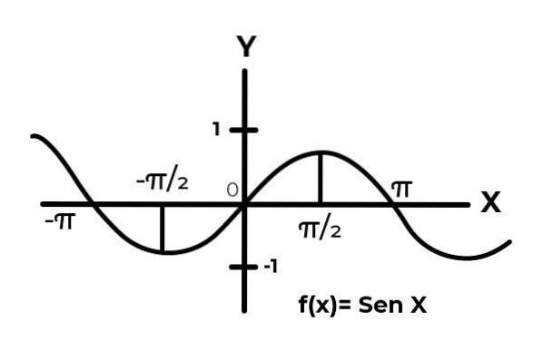
As can be seen in the graph. Start from scratch in x = 0 then reaching a maximum in x = π / 2. It is after x = π / 2 that the values ​​begin to repeat, until they return to zero in x = π. In this way it is known that F (x) = Sen (x) is not injective for the interval [0 , π ] .

When studying the graph of the function F (x) = Sen (x) intervals are observed where the behavior of the curve adapts to the injectivity criteria. As for example the interval  [  π / 2,3π / 2  ]

Where the function varies results from 1 to -1, without repeating any value in the dependent variable.

In this way the function F: [  π / 2,3π / 2  ] → R defined by F (x) = Sen (x). It is injective

Example 6

Check if the function F: [0, ∞) → R defined by F (x) = 3x^two it is injective.

This time the domain of the expression is already limited. It is also observed that the values ​​of the dependent variable do not repeat themselves in this interval.

Therefore, it can be concluded that F: [0, ∞) → R defined by F (x) = 3x^two   it is injective

Example 7

Identify which of the following functions is

1. It is injective. The associated elements of the codomain are unique for each value of the independent variable.
2. It is not injective. There are elements of the codomain associated with more than one element of the starting set.
3. It is injective
4. It is not injective

Proposed exercises for class / home

Check if the following functions are injective:

F: [0, ∞) → R defined by F (x) = (x + 3)^two  

F: [ π / 2,3π / 2  ] → R defined by F (x) = Tan (x)

F: [ -π,π  ] → R defined by F (x) = Cos (x + 1)

F: R → R defined by the line F (x) = 7x + 2

References

1. Introduction to Logic and Critical Thinking. Merrilee H. Salmon. University of Pittsburgh
2. Problems in Mathematical Analysis. Piotr Biler, Alfred Witkowski. University of Wroclaw. Poland.
3. Elements of Abstract Analysis. Mícheál O'Searcoid PhD. Department of mathematics. University college Dublin, Beldfield, Dublind 4.
4. Introduction to Logic and to the Methodology of the Deductive Sciences. Alfred Tarski, New York Oxford. Oxford University press.
5. Principles of mathematical analysis. Enrique Linés Escardó. Editorial Reverté S. A 1991. Barcelona Spain.