
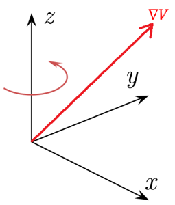
The potential gradient is a vector that represents the rate of change of the electric potential with respect to the distance in each axis of a Cartesian coordinate system. Thus, the potential gradient vector indicates the direction in which the rate of change of the electric potential is greater, as a function of the distance.
In turn, the modulus of the potential gradient reflects the rate of change of the variation of electric potential in a particular direction. If the value of this is known at each point of a spatial region, then the electric field can be obtained from the potential gradient.
The electric field is defined as a vector, thus it has a specific direction and magnitude. By determining the direction in which the electric potential decreases most rapidly - away from the reference point - and dividing this value by the distance traveled, the magnitude of the electric field is obtained.
Article index
The potential gradient is a vector delimited by specific spatial coordinates, which measures the ratio of change between the electric potential and the distance traveled by said potential.
The most outstanding characteristics of the electric potential gradient are detailed below:
1- The potential gradient is a vector. Hence, it has a specific magnitude and direction.
2- Since the potential gradient is a vector in space, it has magnitudes directed on the X (width), Y (height) and Z (depth) axes, if the Cartesian coordinate system is taken as reference.
3- This vector is perpendicular to the equipotential surface at the point at which the electric potential is evaluated.
4- The potential gradient vector is directed towards the direction of maximum variation of the electric potential function at any point.
5- The modulus of the potential gradient is equal to the derivative of the electric potential function with respect to the distance traveled in the direction of each of the axes of the Cartesian coordinate system.
6- The potential gradient has zero value at stationary points (maximums, minimums and saddle points).
7- In the international system of units (SI), the units of measurement of the potential gradient are volts / meters.
8- The direction of the electric field is the same in which the electric potential decreases its magnitude faster. In turn, the potential gradient points in the direction in which the potential increases in value relative to a change in position. So, the electric field has the same value of the potential gradient, but with the opposite sign.
The difference in electric potential between two points (point 1 and point 2), is given by the following expression:
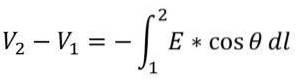
Where:
V1: electric potential at point 1.
V2: electric potential at point 2.
E: magnitude of electric field.
Ѳ: angle the inclination of the measured electric field vector in relation to the coordinate system.
When expressing this formula differentially, the following follows:
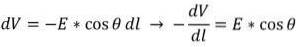
The factor E * cos (Ѳ) refers to the modulus of the electric field component in the direction of dl. Let L be the horizontal axis of the reference plane, then cos (Ѳ) = 1, like this:
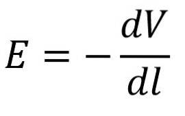
Hereafter, the quotient between the variation in electric potential (dV) and the variation in the distance traveled (ds) is the modulus of the potential gradient for said component.
From there it follows that the magnitude of the electric potential gradient is equal to the component of the electric field in the direction of study, but with the opposite sign.
However, since the real environment is three-dimensional, the potential gradient at a given point must be expressed as the sum of three spatial components on the X, Y, and Z axes of the Cartesian system..
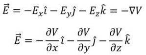
By breaking down the electric field vector into its three rectangular components, we have the following:
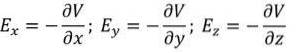
If there is a region in the plane in which the electric potential has the same value, the partial derivative of this parameter with respect to each of the Cartesian coordinates will be zero.
Thus, at points that are on equipotential surfaces, the intensity of the electric field will have zero magnitude.
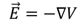
Finally, the potential gradient vector can be defined as exactly the same electric field vector (in magnitude), with the opposite sign. Thus, the following is obtained:
From the previous calculations it is necessary to:
Now, before determining the electric field as a function of the potential gradient, or vice versa, it must first be determined which is the direction in which the electric potential difference grows.
After that, the quotient of the variation of the electric potential and the variation of the net distance traveled is determined.
In this way, the magnitude of the associated electric field is obtained, which is equal to the magnitude of the potential gradient in that coordinate.
There are two parallel plates, as reflected in the following figure.
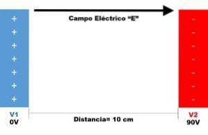
The direction of growth of the electric field is determined on the Cartesian coordinate system.
The electric field grows only in the horizontal direction, given the arrangement of the parallel plates. Consequently, it is feasible to deduce that the components of the potential gradient on the Y axis and the Z axis are zero..
Data of interest is discriminated.
- Potential difference: dV = V2 - V1 = 90 V - 0 V => dV = 90 V.
- Difference in distance: dx = 10 centimeters.
To guarantee the consistency of the measurement units used according to the International System of Units, the quantities that are not expressed in SI must be converted accordingly. Thus, 10 centimeters equals 0.1 meters, and finally: dx = 0.1 m.
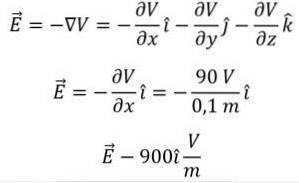
Calculate the magnitude of the potential gradient vector as appropriate.


Yet No Comments