The homoscedasticity in a predictive statistical model it occurs if in all the data groups of one or more observations, the variance of the model with respect to the explanatory (or independent) variables remains constant.
A regression model can be homoscedastic or not, in which case we speak of heteroscedasticity.
A statistical regression model of several independent variables is called homoscedastic, only if the variance of the error of the predicted variable (or the standard deviation of the dependent variable) remains uniform for different groups values of the explanatory or independent variables.
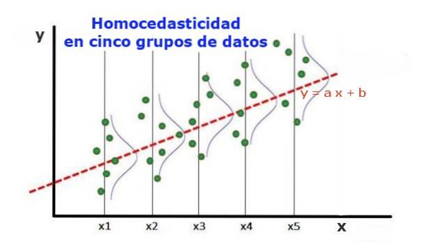
In the five data groups in Figure 1, the variance in each group has been calculated, with respect to the value estimated by the regression, turning out to be the same in each group. It is further assumed that the data follow the normal distribution.
At the graphical level, it means that the points are equally scattered or scattered around the value predicted by the regression fit, and that the regression model has the same error and validity for the range of the explanatory variable..
Article index
To illustrate the importance of homoscedasticity in predictive statistics, it is necessary to contrast with the opposite phenomenon, heteroscedasticity.
In the case of figure 1, in which there is homoscedasticity, it is true that:
Var ((y1-Y1); X1) ≈ Var ((y2-Y2); X2) ≈… Var ((y4-Y4); X4)
Where Var ((yi-Yi); Xi) represents the variance, the pair (xi, yi) represents data from group i, while Yi is the value predicted by the regression for the mean value Xi of the group. The variance of the n data from group i is calculated as follows:
Var ((yi-Yi); Xi) = ∑j (yij - Yi) ^ 2 / n
On the contrary, when heteroscedasticity occurs, the regression model may not be valid for the entire region in which it was calculated. Figure 2 shows an example of this situation.
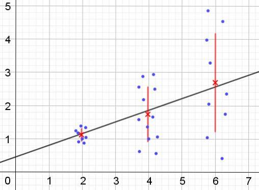
Figure 2 represents three groups of data and the fit of the set using a linear regression. It should be noted that the data in the second and third groups are more dispersed than in the first group. The graph in figure 2 also shows the mean value of each group and its error bar ± σ, with the σ standard deviation of each group of data. It should be remembered that the standard deviation σ is the square root of the variance.
It is clear that in the case of heteroscedasticity, the regression estimation error is changing in the range of values of the explanatory or independent variable, and in the intervals where this error is very large, the regression prediction is unreliable or unreliable. not applicable.
In a regression model the errors or residuals (and -Y) must be distributed with equal variance (σ ^ 2) throughout the interval of values of the independent variable. It is for this reason that a good regression model (linear or nonlinear) must pass the homoscedasticity test..
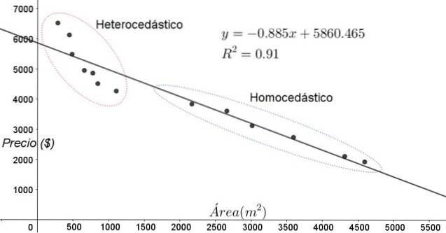
The points shown in figure 3 correspond to the data of a study that looks for a relationship between the prices (in dollars) of the houses as a function of the size or area in square meters.
The first model to be tested is that of a linear regression. First of all, it is noted that the coefficient of determination R ^ 2 of the fit is quite high (91%), so it can be thought that the fit is satisfactory..
However, two regions can be clearly distinguished from the adjustment graph. One of them, the one on the right enclosed in an oval, fulfills homoscedasticity, while the region on the left does not have homoscedasticity.
This means that the prediction of the regression model is adequate and reliable in the range from 1800 m ^ 2 to 4800 m ^ 2 but very inadequate outside this region. In the heteroscedastic zone, not only is the error very large, but also the data seem to follow a different trend than the one proposed by the linear regression model..
The scatter plot of the data is the simplest and most visual test of their homoscedasticity, however on occasions where it is not as evident as in the example shown in figure 3, it is necessary to resort to graphs with auxiliary variables..
In order to separate the areas where homoscedasticity is fulfilled and where it is not, the standardized variables ZRes and ZPred are introduced:
ZRes = Abs (y - Y) / σ
ZPred = Y / σ
It should be noted that these variables depend on the applied regression model, since Y is the value of the regression prediction. Below is the scatter plot ZRes vs ZPred for the same example:
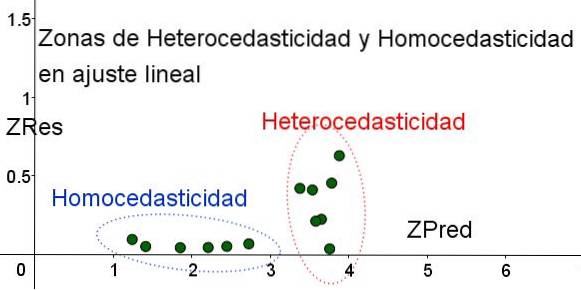
In the graph in Figure 4 with the standardized variables, the area where the residual error is small and uniform is clearly separated from the area where it is not. In the first zone, homoscedasticity is fulfilled, while in the region where the residual error is highly variable and large, heteroscedasticity is fulfilled..
Regression adjustment is applied to the same group of data in figure 3, in this case the adjustment is non-linear, since the model used involves a potential function. The result is shown in the following figure:
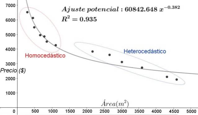
In the graph in Figure 5, the homoscedastic and heteroscedastic areas should be clearly noted. It should also be noted that these areas were interchanged with respect to those that were formed in the linear fit model.
In the graph of figure 5 it is evident that even when there is a fairly high coefficient of determination of the fit (93.5%), the model is not adequate for the entire interval of the explanatory variable, since the data for greater than 2000 m ^ 2 present heteroskedasticity.
One of the non-graphical tests most used to verify whether homoscedasticity is fulfilled or not is the Breusch-Pagan test.
Not all the details of this test will be given in this article, but its fundamental characteristics and the steps of the same are outlined in broad strokes:
Most of the statistical software packages such as: SPSS, MiniTab, R, Python Pandas, SAS, StatGraphic and several others incorporate the homoscedasticity test of Breusch-Pagan. Another test to verify uniformity of variance the Levene's test.


Yet No Comments