Block algebra elements, examples, solved exercises

The block algebra refers to the set of operations that are executed through blocks. These and some other elements serve to schematically represent a system and easily visualize its response to a given input..

In general, a system contains various electrical, electronic and electromechanical elements, and each one of them, with its respective function and position in the system, as well as the way they are related, is outlined through functional blocks.

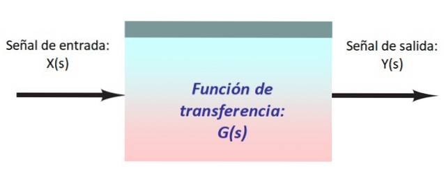
In the figure above there is a very simple system, which consists of an input signal X (s), which enters the block with the transfer function G (s) that modifies it and produces the output Y (s).

It is convenient to represent the signals and their path through the system by means of arrows that enter and leave each block. Usually the signal flow is directed from left to right.

The advantage of this kind of schematic is the visual aid it provides in understanding the system, even if it is not a physical representation of the system. In fact, the block diagram is not unique, because depending on the point of view, several diagrams of the same system can even be drawn..

It can also happen that the same diagram serves several systems that are not necessarily related to each other, as long as it adequately describes their behavior. There are different systems whose response is similar in many respects, for example an LC circuit (inductor-capacitor) and a mass-spring system..

Article index

• 1 What is a block diagram?
• 2 Elements of the block diagram
  • 2.1 The signal
  • 2.2 The block
  • 2.3 Sum point
  • 2.4 Branch point
• 3 Examples of block algebra rules
  • 3.1 Cascading blocks
  • 3.2 Blocks in parallel
  • 3.3 Move an adder to the left
  • 3.4 Move an adder to the right
  • 3.5 Moving a branching point from left to right
  • 3.6 Move a branching point from right to left
  • 3.7 Feedback system
  • 3.8 System with feedback and transducer
• 4 Solved exercises
  • 4.1 Exercise 1
  • 4.2 Exercise 2
• 5 References

What is a block diagram?

The systems are generally more complicated than the one in figure 1, but block algebra provides a series of simple rules to manipulate the scheme of the system and reduce it to its simplest version..

As explained at the beginning, the diagram uses blocks, arrows and circles to establish the relationship between each component of the system and the flow of signals that run through it..

Block algebra allows you to compare two or more signals by adding, subtracting and multiplying them, as well as analyzing the contribution that each component makes to the system.

Thanks to this it is possible to reduce the entire system to a single input signal, a single transfer function that fully describes the action of the system and the corresponding output..

Block diagram elements

The elements of the block diagram are as follows:

The signal

The signals are of a very varied nature, for example it is common for it to be an electric current or a voltage, but it can be light, sound and more. The important thing is that it contains information about a certain system.

The signal is denoted with a capital letter if it is a function of the variable s of the Laplace transform: X (s) (see figure 1) or with lowercase if it is a function of time t, as x (t).

In the block diagram, the input signal is represented by an arrow directed towards the block, while the output signal, denoted as Y (s) or y (t), is indicated by an outgoing arrow.

Both the input and output signals are unique and the direction the information flows is determined by the direction of the arrow. And the algebra is the same for either of the two variables.

The block

The block is represented by a square or a rectangle (see figure 1) and can be used to carry out operations or implement the transfer function, which is usually denoted by the capital letter G. This function is a mathematical model using which describes the response offered by the system to an input signal.

The transfer function can be expressed in terms of time t as G (t) or the variable s as G (s).

When the input signal X (s) reaches the block, it is multiplied by the transfer function and transformed into the output signal Y (s). Mathematically it is expressed like this:

Y (s) = X (s) .G (s)

Equivalently, the transfer function is the ratio between the Laplace transform of the output signal and the Laplace transform of the input signal, provided that the initial conditions of the system are null:

G (s) = Y (s) / X (s)

Sum point

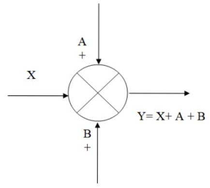
The addition point, or adder, is symbolized by a circle with a cross inside. It is used to combine, by means of addition and subtraction, two or more signals. At the end of the arrow that symbolizes the signal, a + sign is placed directly if said signal is added or a - sign if it is subtracted.

In the following figure there is an example of how the adder works: we have the input signal X, to which the signals A and B are added, obtaining as a result the output Y, which is algebraically equivalent to:

Y = X + A + B

Branch point

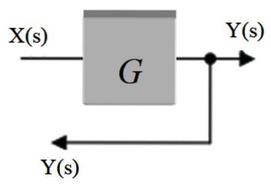
It's also called bifurcation point. In it, the signal that comes out of a block is distributed to other blocks or to an adder. It is represented by a point placed on the signal arrow and another arrow comes out of it that redirects the signal to another part.

Examples of block algebra rules

As explained before, the idea is to express the system using the block diagram and reduce it to find the transfer function that describes it. The following are the block algebra rules to simplify diagrams:

Cascading blocks

When you have a signal that passes successively through the G blocks₁, G_two, G₃..., is reduced to a single block whose transfer function is the product of G₁, G_two, G₃...

In the following example, the signal X (s) enters the first block and its output is:

Y₁(s) = X (s) .G₁(s)

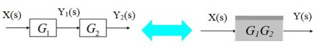
Turn Y₁(s) enter block G_two(s), whose output is:

Y_two(s) = X (s) .G₁(s). G_two(s)

The procedure is valid for n cascaded blocks:

Y_n (s) = X (s). G₁(s) .G_two(s) ... G_n(s)

Parallel blocks

In the diagram on the left, the signal X (s) branches to enter the G blocks₁(s) and G_two(s):

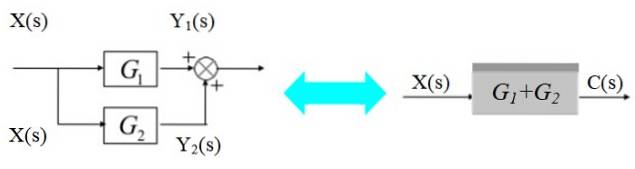
The respective output signals are:

Y₁(s) = X (s) .G₁(s)

Y_two(s) = X (s) .G_two(s)

These signals are added together to obtain:

C (s) = Y₁(s) + Y_two(s) = X (s). [G₁(s) + G_two(s)]

As shown in the diagram to the right.

Move an adder to the left

An adder can be shifted to the left of the block as follows:

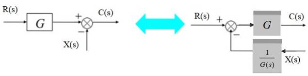
On the left the output signal is:

C (s) = R (s). G (s) - X (s)

Equivalently to the right:

C (s) = [R (s) - X (s) / G (s)]. G (s)

Move an adder to the right

The adder can be moved to the right of the block like this:

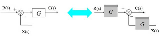
On the left we have: [R (s) - X (s)]. G (s) = C (s)

And on the right:

R (s). G (s) - X (s). G (s) = C (s)

Move a branching point from left to right

To move the branching point from left to right of the block, just observe that the output C (s) to the right is the product X (s) .G (s). Since you want to convert it to X (s) again, multiply by the inverse of G (s).

Move a branching point from right to left

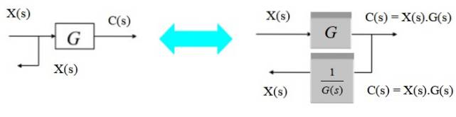
Alternatively the branching point can be shifted from right to left as follows:

Since at the exit of the branch we want to obtain C (s), simply insert a new block G (s) at a branch point to the left of the original block.

Feedback system

In the following system the output signal C (s) is fed back through the adder on the left:

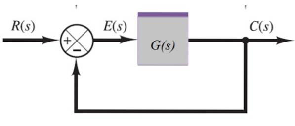
C (s) = E (s) .G (s)

But:

E (s) = R (s) -C (s)

Substituting this expression in the previous equation it remains: C (s) = [R (s) -C (s)]. G (s), from which C (s) can be solved:

C (s) + C (s) .G (s) = R (s) .G (s) → C (s). [1 + G (s)] = R (s) .G (s)

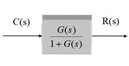
C (s) = R (s). G (s) / [1 + G (s)]

Or alternatively:

C (s) / R (s) = G (s) / [1 + G (s)]

In graphical form, after simplifying it remains:

System with feedback and transducer

The transducer consists of the transfer function H (s):

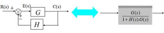
In the diagram to the right, the output signal C (s) is:

C (s) = E (s). G (s) with E (s) = R (s) - C (s). H (s)

Then:

C (s) = [R (s) - C (s). H (s)]. G (s)

C (s) [1+ H (s) .G (s)] = R (s) .G (s)

Therefore, C (s) can be solved by:

C (s) = G (s) .R (s) / [1+ H (s) .G (s)]

And the transfer function will be:

G (s) / [1+ H (s) .G (s)]

As shown in the simplified diagram to the right.

Solved exercises

Exercise 1

Find the transfer function of the following system:

Solution

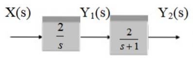
It treats two blocks in cascade, therefore the transfer function is the product of the functions G₁ and G_two.

It has to:

G₁ = 2 / s

G_two = 2 / (s + 1)

Therefore the transfer function sought is:

G (s) = 4 / [s (s + 1)]

Exercise 2

Reduce the following system:

Solution

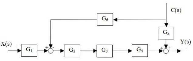
First the G cascade is reduced_two, G₃ and G_4, and the parallel G is separated₅ and G₆:

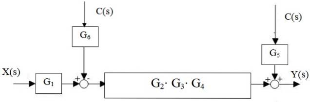
Then the adder to the left of block G_two ⋅G₃ ⋅ G₄ moves to the right:

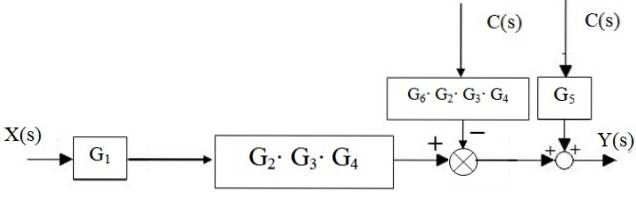
The adders on the right are reduced to just one, as well as the cascading blocks:

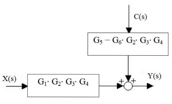
Finally, the output of the system is:

Y (s) = X (s) ⋅G₁⋅ G_two ⋅G₃ ⋅ G₄ + C (s) ⋅ [G₅ - G₆ ⋅ G_two ⋅G₃ ⋅ G₄]

References

1. Alaydi, J. Control system block diagram. Recovered from: site.iugaza.edu.ps.
2. Bolton, W. 2006. Control engineering. 2nd. Edition. Alpha Omega.
3. Cwalinsky, J. Introduction to system block algebra. Recovered from: cedengineering.com.
4. Dademuchconnection. Blocks diagram. Recovered from: dademuch.com.
5. Ogata, K. 2010. Modern control engineering. 5th. Edition. Pearson.