The approximate measurement of amorphous figures consists of a series of methods used to determine the area or perimeter of geometric figures that are not triangles, squares, circles, etc. Some are extendable to three-dimensional figures.
Basically the measurement consists of making a grid of some regular shape, such as rectangles, squares or trapezoids, that approximately cover the surface. The precision of the approximation of the area obtained by these methods increases with the fineness or density of the lattice..
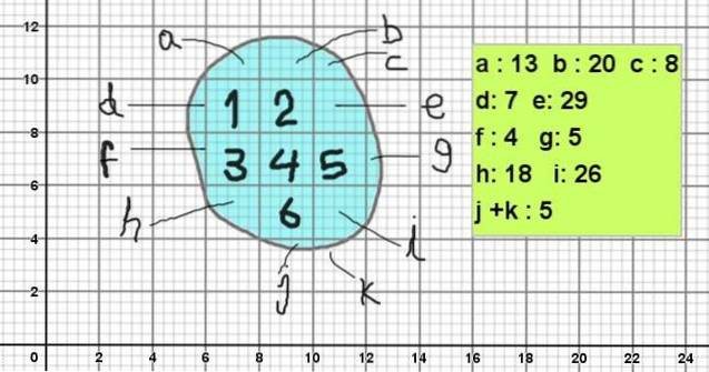
Figures 1 and 2 show various amorphous figures. To calculate the area, a grid has been made, composed of 2 X 2 squares, which in turn are subdivided into twenty-five 2/5 x 2/5 squares.
Adding the areas of the main squares and the secondary squares gives the approximate area of the amorphous figure.
Article index
It is often necessary to roughly calculate the area under a curve between two limit values. In this case, instead of a square lattice, rectangular stripes can be drawn that roughly cover the area under the said curve..
The sum of all the rectangular stripes is called sum or Riemann sum. Figure 3 shows a partition of the interval [a, b] over which the area under the curve is to be approximated..
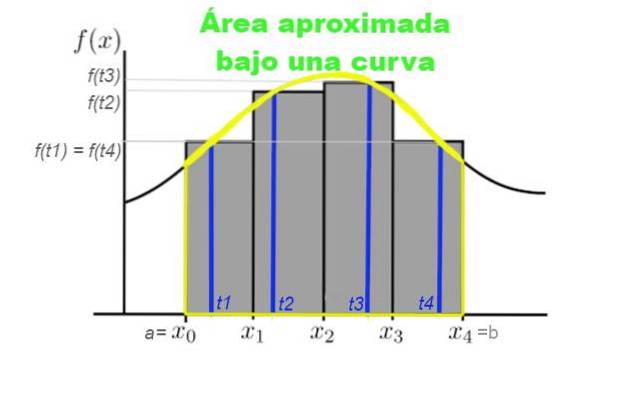
Suppose you want to calculate the area under the curve given by the function y = f (x), where x belongs to the interval [a, b] within which you want to calculate the area. For this, a partition of n elements is made within this interval:
Partition = x0 = a, x1, x2,…, xn = b.
Then the approximate area under the curve given by y = f (x) in the interval [a, b] is obtained by carrying out the following summation:
S = ∑k = 1n f (tk) (xk - xk-1)
Where Tk is between xk-1 and xk: xk-1 ≤ tk ≤ xk .
Figure 3 graphically shows the Riemann sum of the curve y = f (x) in the interval [x0, x4]. In this case, a partition of four subintervals was made and the sum represents the total area of the gray rectangles.
This sum represents an approximation to the area under the curve f between the abscissa x = x0 and x = x4.
The approximation to the area under the curve improves as the number n of partitions is larger, and tends to be exactly the area under the curve when the number n of partitions tends to infinity.
In case the curve is represented by an analytical function, the values f (tk) are calculated by evaluating this function at the t valuesk. But if the curve does not have an analytic expression, then the following possibilities remain:
Depending on the choice of the value tk in the interval [xk, xk-1], the sum can overestimate or underestimate the exact value of the area under the curve of the function y = f (x). The most advisable thing is to take the point tk where the missing area is approximately equal to the excess area, although it is not always possible to make such a choice..
The most practical thing then is to use regular intervals of width Δx = (b - a) / n, where a and b are the minimum and maximum values of the abscissa, while n is the number of subdivisions.
In that case the area under the curve is approximated by:
Area = f (a + Δx) + f (a + 2Δx) +… + f [a + (n-1] Δx + f (b) * Δx
In the above expression, tk was taken at the right end of the subinterval.
Another practical possibility is to take the value tk at the extreme left, in which case the sum that approximates the area is expressed as:
Area = [f (a) + f (a + Δx) +… + f (a + (n-1) Δx)] * Δx
In case tk is chosen as the central value of the regular subinterval of width Δx, the sum that approximates the area under the curve is:
Area = [f (a + Δx / 2) + f (a + 3Δx / 2) +… + f (b- Δx / 2)] * Δx
Any of these expressions tends to the exact value to the extent that the number of subdivisions is arbitrarily large, that is, that Δx tends to zero, but in this case the number of terms in the summation becomes immensely large with the consequent computational cost.
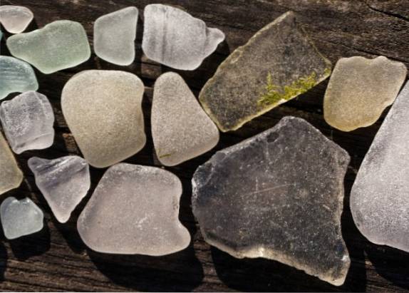
Figure 2 shows an amorphous figure, whose contour is similar to the stones in image 1. To calculate its area, it is placed on a grid with main squares of 2 x 2 squared units (for example, they can be 2 cm²)..
And since each square is subdivided into 5 x 5 subdivisions, then each subdivision has an area of 0.4 x 0.4 squared units (0.16 cm²).
The area of the figure would be calculated like this:
Area = 6 x 2 cm² + (13 + 20 + 8 + 7 + 29 + 4 + 5 + 18 + 26 + 5) x 0.16 cm²
Namely:
Area = 12 cm² + 135 x 0.16 cm² = 33.6 cm².
Calculate approximately the area under the curve given by the function f (x) = xtwo between a = -2 through b = +2. To do this, first write the sum for n regular partitions of the interval [a, b] and then take the mathematical limit for the case that the number of partitions tends to infinity.
First define the interval of the partitions as
Δx = (b - a) / n.
Then the right sum corresponding to the function f (x) looks like this:

[-2 + (4i / n)]two = 4 - 16 i / n + (4 / n)two itwo
And then it is substituted in the summation:
And the third results:
S (f, n) = 16 - 64 (n + 1) / 2n + 64 (n + 1) (2n + 1) / 6ntwo
Choosing a large value for n gives a good approximation to the area under the curve. However, in this case it is possible to get the exact value by taking the mathematical limit when n tends to infinity:
Area = limn-> ∞[16 - 64 (n + 1) / 2n + 64 (n + 1) (2n + 1) / 6ntwo]
Area = 16 - (64/2) + (64/3) = 16/3 = 5,333.

Yet No Comments