
The dynamic programming is an algorithm model that solves a complex problem by dividing it into subproblems, storing their results in order to avoid having to recalculate those results.
This schedule is used when you have problems that can be divided into similar subproblems, so that their results can be reused. For the most part, this programming is used for optimization.
Before solving the available subproblem, the dynamic algorithm will attempt to examine the results of the previously solved subproblems. Subproblem solutions are combined to achieve the best solution.
Instead of calculating the same subproblem over and over again, you can store your solution in some memory, when you first encounter this subproblem. When it appears again during the solution of another subproblem, the solution already stored in memory will be taken.
This is a wonderful idea to fix time with memory, where by using additional space you can improve the time required to find a solution..
Article index
The following essential characteristics are what you must have a problem with before dynamic programming can be applied:
This characteristic expresses that an optimization problem can be solved by combining the optimal solutions of the secondary problems that comprise it. These optimal substructures are described by recursion.
For example, in a graph an optimal substructure will be presented in the shortest path r that goes from a vertex s to a vertex t:
That is, in this shortest path r any intermediate vertex i can be taken. If r is really the shortest route, then it can be divided into the sub-routes r1 (from s to i) and r2 (from i to t), in such a way that these are in turn the shortest routes between the corresponding vertices.
Therefore, to find the shortest routes, the solution can be easily formulated recursively, which is what the Floyd-Warshall algorithm does..
The subproblem space must be small. That is, any recursive algorithm that solves a problem will have to solve the same subproblems over and over again, instead of generating new subproblems..
For example, to generate the Fibonacci series we can consider this recursive formulation: Fn = F (n-1) + F (n-2), taking as a base case that F1 = F2 = 1. Then we will have: F33 = F32 + F31, and F32 = F31 + F30.
As you can see, F31 is being resolved into the recursive subtrees of both F33 and F32. Although the total number of subproblems is really small, if you adopt a recursive solution like this you will end up solving the same problems over and over again..
This is taken into account by dynamic programming, so it solves each subproblem only once. This can be accomplished in two ways:
If the solution to any problem can be recursively formulated using the solution of its subproblems, and if these subproblems overlap, then the solutions to the subproblems can be easily memorized or stored in a table.
Each time a new subproblem solution is sought, the table will be checked to see if it was previously solved. If a solution is stored, it will be used instead of calculating it again. Otherwise, the subproblem will be solved, storing the solution in the table.
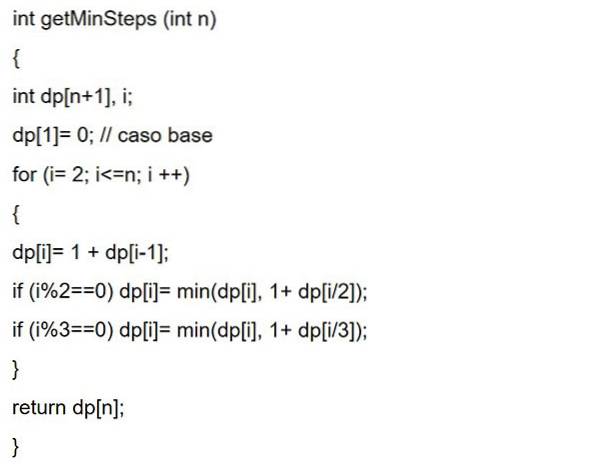
After the solution of a problem is recursively formulated in terms of its subproblems, it will be possible to try to reformulate the problem in an ascending way: first we will try to solve the subproblems and use their solutions to arrive at solutions to the larger subproblems..
This is also generally done in table form, iteratively generating solutions to larger and larger subproblems by using solutions to smaller subproblems. For example, if the values of F31 and F30 are already known, the value of F32 can be calculated directly.
One significant feature of a problem that can be solved through dynamic programming is that it should have subproblems overlapping. This is what distinguishes dynamic programming from the divide and conquer technique, where it is not necessary to store the simplest values.
It is similar to recursion, since when calculating the base cases the final value can be determined inductively. This bottom-up approach works well when a new value depends only on previously calculated values.
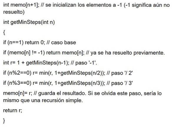
For any positive integer "e", any of the following three steps can be performed.
- Subtract 1 from the number. (e = e-1).
- If it is divisible by 2, divide by 2 (if e% 2 == 0, then e = e / 2).
- If it is divisible by 3, divide by 3 (if e% 3 == 0, then e = e / 3).
Based on the steps above, the minimum number of these steps must be found to bring e to 1. For example:
- If e = 1, result: 0.
- If e = 4, result: 2 (4/2 = 2/2 = 1).
- When e = 7, result: 3 (7-1 = 6/3 = 2/2 = 1).
One might think of always choosing the step that makes n as low as possible and continuing like this, until it reaches 1. However, it can be seen that this strategy does not work here..
For example, if e = 10, the steps would be: 10/2 = 5-1 = 4/2 = 2/2 = 1 (4 steps). However, the optimal form is: 10-1 = 9/3 = 3/3 = 1 (3 steps). Therefore, all possible steps that can be done for each value of n found should be tried, choosing the minimum number of these possibilities.
Everything starts with recursion: F (e) = 1 + min F (e-1), F (e / 2), F (e / 3) if e> 1, taking as base case: F (1) = 0. Having the recurrence equation, you can start to code the recursion.
However, it can be seen that it has overlapping subproblems. Furthermore, the optimal solution for a given input depends on the optimal solution of its subproblems.
As in memorization, where the solutions of the subproblems that are solved are stored for later use. Or as in dynamic programming, you start at the bottom, working your way up to the given e. Then both codes:
One of the main advantages of using dynamic programming is that it speeds up the processing, since references that were previously calculated are used. As it is a recursive programming technique, it reduces the lines of code of the program.
Greedy algorithms are similar to dynamic programming in that they are both tools for optimization. However, the greedy algorithm looks for an optimal solution at each local step. That is, it seeks a greedy choice in the hope of finding a global optimum..
Therefore, greedy algorithms can make an assumption that looks optimal at the time, but becomes expensive in the future and does not guarantee a global optimum..
On the other hand, dynamic programming finds the optimal solution for the subproblems and then makes an informed choice by combining the results of those subproblems to actually find the most optimal solution..
- Much memory is needed to store the calculated result of each subproblem, unable to guarantee that the stored value will be used or not.
- Many times, the output value is stored without ever being used in the following subproblems during execution. This leads to unnecessary memory usage.
- In dynamic programming functions are called recursively. This keeps the stack memory constantly increasing.
If you have limited memory to run your code and processing speed is not a concern, you can use recursion. For example, if you are developing a mobile application, the memory is very limited to run the application.
If you want the program to run faster and you do not have memory restrictions, it is preferable to use dynamic programming.
Dynamic programming is an effective method of solving problems that might otherwise seem extremely difficult to solve in a reasonable amount of time..
Algorithms based on the dynamic programming paradigm are used in many areas of science, including many examples in artificial intelligence, from planning problem solving to speech recognition..
Dynamic programming is quite effective and works very well for a wide range of problems. Many algorithms can be seen as greedy algorithm applications, such as:
- Fibonacci number series.
- Hanoi Towers.
- All shortest route pairs by Floyd-Warshall.
- Backpack problem.
- Project scheduling.
- The shortest way through Dijkstra.
- Flight control and robotics control.
- Mathematical optimization problems.
- Timesharing - Schedule the job to maximize CPU usage.
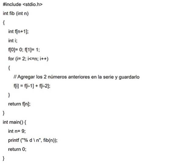
Fibonacci numbers are the numbers found in the following sequence: 0, 1, 1, 2, 3, 5, 8, 13, 21, 34, 55, 89, 144, etc..
In mathematical terminology, the sequence Fn of Fibonacci numbers is defined by the recurrence formula: F (n) = F (n -1) + F (n -2), where F (0) = 0 and F ( 1) = 1.
In this example, a search array with all initial values is initialized with -1. Whenever the solution to a subproblem is needed, this search matrix will be searched first.
If the calculated value is there, then that value will be returned. Otherwise, the result will be calculated to be stored in the search matrix so that it can be reused later.
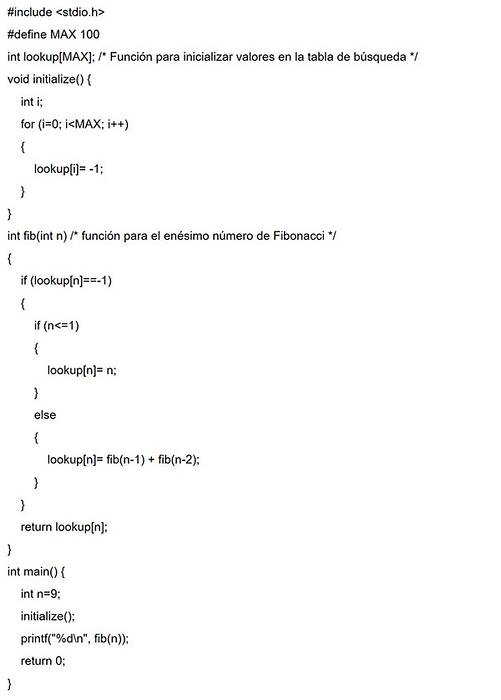
In this case, for the same Fibonacci series, f (0) is calculated first, then f (1), f (2), f (3), and so on. Thus, the solutions of the subproblems will be constructed from the bottom up.


Yet No Comments