The Continuous variable It is one that can take an infinite number of numerical values between two given values, even if those two values are arbitrarily close. They are used to describe measurable attributes; for example height and weight. The values that a continuous variable takes can be rational numbers, real numbers or complex numbers, although the latter case is less frequent in statistics.
The main characteristic of continuous variables is that between two rational or real values another can always be found, and between that other and the first another value can be found, and so on indefinitely..

For example, suppose the variable weight in a group where the heaviest weighs 95 kg and the lowest weighs 48 kg; that would be the range of the variable and the number of possible values is infinite.
For example between 50.00 kg and 50.10 kg can be 50.01. But between 50.00 and 50.01 can be the measure 50.005. That is a continuous variable. On the other hand, if a precision of a single decimal were established in the possible measures of weight, then the variable used would be discrete.
Continuous variables belong to the category of quantitative variables, because they have a numerical value associated with them. With this numerical value it is possible to perform mathematical operations ranging from arithmetic to infinitesimal calculation methods..
Article index
Most of the variables in physics are continuous variables, among them we can name: length, time, speed, acceleration, energy, temperature and others.
In statistics, various types of variables can be defined, both qualitative and quantitative. Continuous variables belong to the latter category. With them it is possible to carry out arithmetic and calculation operations.
For example the variable h, corresponding to people with height between 1.50 m and 1.95 m, it is a continuous variable.
Let's compare this variable with this other: the number of times a coin flips heads, which we will call n.
The variable n can take values between 0 and infinity, however n It is not a continuous variable since it cannot take the value 1.3 or 1.5, because between values 1 and 2 there is no other. This is an example of discrete variable.
Consider the following example: a machine produces matchsticks and packs them in its box. Two statistical variables are defined:
Variable 1: L = Length of the match.
Variable 2: N = Number of matches per box.
The nominal match length is 5.0 cm with a tolerance of 0.1 cm. The number of matches per box is 50 with a tolerance of 3.
a) Indicate the range of values that can take L Y N.
b) How many values can it take L?
c) How many values can it take n?
Say in each case if it is a discrete or continuous variable.
The values of L are in the range [5.0-0.1; 5.0 + 0.1]; that is to say that the value of L is in the range [4.9 cm; 5.1 cm] and the variable L it can take infinite values between these two measures. It is then a continuous variable.
The value of the variable n is in the interval [47; 53]. The variable n it can only take 6 possible values in the tolerance interval, it is then a discrete variable.
If, in addition to being continuous, the values taken by the variable have a certain probability of occurrence associated with them, then it is a continuous random variable. It is very important to distinguish if the variable is discrete or continuous, since the probabilistic models applicable to one and the other are different..
A continuous random variable is completely defined when the values that it can assume are known, and the probability that each of them has of happening.
The matchmaker makes them in such a way that the length of the sticks is always between the values 4.9 cm and 5.1 cm, and zero outside these values. There is the probability of obtaining a stick that measures between 5.00 and 5.05 cm, although we could also extract one of 5,0003 cm. Are these values equally likely?.
Suppose the probability density is uniform. The probabilities of finding a match with a certain length are listed below:
-That a phosphor is in the range [4,9; 5.1] has probability = 1 (or 100%), since the machine does not draw matches outside of these values.
-Finding a match that is between 4.9 and 5.0 has probability = ½ = 0.5 (50%), since it is half the range of lengths.
-And the probability that the match has length between 5.0 and 5.1 is also 0.5 (50%)
-It is known that there are no match sticks that are between 5.0 and 5.2 in length. Probability: zero (0%).
Now let us observe the following probabilities P of obtaining sticks whose length is between l1 and ltwo:
P = (ltwo -l1) / (Lmax - Lmin)
-P for a match to have a length between 5.00 and 5.05 is denoted as P ([5.00, 5.05]):
P ([5.00, 5.05]) = (5.05 - 5.00) / (5.1 - 4.9) = 0.05 / 0.2 = ¼ = 0.25 (25%)
-P that the hill has length between 5.00 and 5.01 is:
P ([5.00, 5.01]) = (5.00 - 5.01) / (5.1 - 4.9) = 0.01 / 0.2 = 1/20 = 0.05 (5 %)
-P that the hill has length between 5,000 and 5,001 is even less:
P (5,000; 5.001) = 0.001 / 0.2 = 1/200 = 0.005 (0.5%)
If we keep decreasing the interval to get closer and closer to 5.00, the probability that a toothpick is exactly 5.00 cm is zero (0%). What we do have is the probability of finding a match within a certain range.
If the events are independent, the probability that two toothpicks are in a certain range is the product of their probabilities.
-The probability that two toothpicks are between 5.0 and 5.1 is 0.5 * 0.5 = 0.25 (0.25%)
-The probability that 50 toothpicks are between 5.0 and 5.1 is (0.5) ^ 50 = 9 × 10 ^ -16, that is almost zero.
-The probability that 50 toothpicks are between 4.9 and 5.1 is (1) ^ 50 = 1 (100%)
In the previous example, the assumption was made that the probability is uniform in the given interval, however this is not always the case.
In the case of the actual machine that produces the toothpicks, the chance that the toothpick is at the center value is greater than it is at one of the extreme values. From a mathematical point of view this is modeled with a function f (x) known as probability density.
The probability that the measure L is between a and b is calculated by the definite integral of the function f (x) between a and b.
As an example suppose that we want to find the function f (x), which represents a uniform distribution between the values 4.9 and 5.1 of exercise 1.
If the probability distribution is uniform, then f (x) is equal to the constant c, which is determined by taking the integral between 4.9 and 5.1 of c. Since this integral is the probability, then the result must be 1.
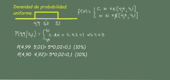
Which means that c is worth 1 / 0.2 = 5. That is, the uniform probability density function is f (x) = 5 if 4.9≤x≤5.1 and 0 outside of this range. Figure 2 shows a uniform probability density function.
Note how in intervals of the same width (for example 0.02) the probability is the same in the center as at the end of the range of the continuous variable L (length of toothpick).
A more realistic model would be a probability density function like the following:
-f (x) = - 750 ((x-5,0) ^ 2-0.01) if 4.9≤x≤5.1
-0 out of this range
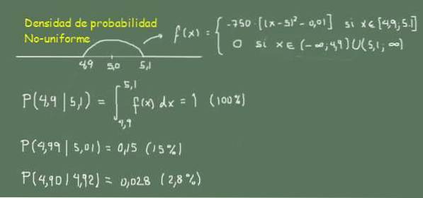
In figure 3 it can be seen how the probability of finding toothpicks between 4.99 and 5.01 (width 0.02) is greater than that of finding toothpicks between 4.90 and 4.92 (width 0.02)


Yet No Comments