The law of Hardy-Weinberg, Also called the Hardy-Weinberg principle or equilibrium, it consists of a mathematical theorem that describes a hypothetical diploid population with sexual reproduction that is not evolving - allele frequencies do not change from generation to generation.
This principle assumes five conditions necessary for the population to remain constant: absence of gene flow, absence of mutations, random mating, absence of natural selection, and an infinitely large population size. In this way, in the absence of these forces, the population remains in equilibrium.
When any of the above assumptions is not met, change occurs. For this reason, natural selection, mutation, migrations, and genetic drift are the four evolutionary mechanisms..
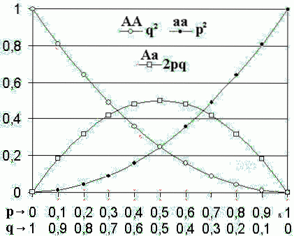
According to this model, when the allele frequencies of a population are p Y what, genotype frequencies will be ptwo, twopq Y whattwo.
We can apply the Hardy-Weinberg equilibrium in calculating the frequencies of certain alleles of interest, for example, to estimate the proportion of heterozygotes in a human population. We can also verify whether or not a population is in equilibrium and propose hypotheses that forces are acting on that population..
Article index
The Hardy-Weinberg principle was born in 1908 and owes its name to its scientists G.H. Hardy and W. Weinberg, who independently reached the same conclusions.
Before that, another biologist named Udny Yule had tackled the problem in 1902. Yule started with a set of genes in which the frequencies of both alleles were 0.5 and 0.5. The biologist showed that the frequencies were maintained during the following generations.
Although Yule concluded that allele frequencies could be kept stable, his interpretation was too literal. He believed that the only state of equilibrium was found when the frequencies corresponded to the value of 0.5.
Yule heatedly discussed her novel findings with R.C. Punnett - widely known in the field of genetics for the invention of the famous "Punnett square." Although Punnett knew that Yule was wrong, he did not find a mathematical way to prove it..
Therefore, Punnett contacted his mathematician friend Hardy, who managed to solve it immediately, repeating the calculations using general variables, and not the fixed value of 0.5 as Yule had done..
Population genetics aims to study the forces that lead to changes in allelic frequencies in populations, integrating Charles Darwin's theory of evolution by natural selection and Mendelian genetics. Today, its principles provide the theoretical basis for understanding many aspects of evolutionary biology..
One of the crucial ideas of population genetics is the relationship between changes in the relative abundance of traits and changes in the relative abundance of the alleles that regulate it, explained by the Hardy-Weinberg principle. In fact, this theorem provides the conceptual framework for population genetics..
In the light of population genetics, the concept of evolution is as follows: change in allele frequencies over generations. When there is no change, there is no evolution.
The Hardy-Weinberg equilibrium is a null model that allows us to specify the behavior of gene and allelic frequencies across generations. In other words, it is the model that describes the behavior of genes in populations, under a series of specific conditions..
In the Hardy-Weinbergm theorem the allelic frequency of TO (dominant allele) is represented by the letter p, while the allelic frequency of to (recessive allele) is represented by the letter what.
The expected genotype frequencies are ptwo, twopq Y whattwo, for the dominant homozygous (AA), heterozygous (Aa) and homozygous recessive (aa), respectively.
If there are only two alleles at that locus, the sum of the frequencies of the two alleles must necessarily equal 1 (p + q = 1). The binomial expansion (p + q)two represent genotype frequencies ptwo + twopq + qtwo = 1.
In a population, the individuals that comprise it interbreed to give rise to offspring. In general, we can point out the most important aspects of this reproductive cycle: the production of gametes, their fusion to give rise to a zygote, and the development of the embryo to give rise to the new generation..
Imagine that we can trace the Mendelian gene process in the events mentioned. We do this because we want to know if and why an allele or genotype will increase or decrease in frequency..
To understand how gene and allele frequencies vary in a population, we will follow the gamete production of a set of mice. In our hypothetical example, mating occurs randomly, where all the sperm and eggs are randomly mixed..
In the case of mice, this assumption is not true and is just a simplification to facilitate calculations. However, in some animal groups, such as certain echinoderms and other aquatic organisms, gametes are expelled and collide randomly..
Now, let's focus our attention on a specific locus, with two alleles: TO Y to. Following the law enunciated by Gregor Mendel, each gamete receives an allele from locus A. Suppose that 60% of the ovules and sperm receive the allele TO, while the remaining 40% received the allele to.
Hence, the allele frequency TO is 0.6 and that of the allele to is 0.4. This group of gametes will be found at random to give rise to a zygote. What is the probability that they will form each of the three possible genotypes? To do this, we must multiply the probabilities as follows:
Genotype AA: 0.6 x 0.6 = 0.36.
Genotype Aa: 0.6 x 0.4 = 0.24. In the case of the heterozygote, there are two forms in which it can originate. The first that the sperm carries the allele TO and the ovule the allele to, or the reverse case, the sperm the to and the ovum TO. Therefore we add 0.24 + 0.24 = 0.48.
Genotype aa: 0.4 x 0.4 = 0.16.
Now, let's imagine that these zygotes develop and become adult mice that will again produce gametes, would we expect the allele frequencies to be the same or different from the previous generation?
Genotype AA will produce 36% of gametes, while heterozygotes will produce 48% of gametes, and the genotype aa 16%.
To calculate the new allele frequency, we add the frequency of the homozygous plus half of the heterozygote, as follows:
Allele frequency TO: 0.36 + ½ (0.48) = 0.6.
Allele frequency to: 0.16 + ½ (0.48) = 0.4.
If we compare them with the initial frequencies, we will realize that they are identical. Therefore, according to the concept of evolution, as there are no changes in allele frequencies over generations, the population is in equilibrium - it does not evolve..
What conditions must the previous population meet so that its allele frequencies remain constant over the generations? In the Hardy-Weinberg equilibrium model, the population that does not evolve meets the following assumptions:
Population must be extremely large in size to avoid stochastic or random effects of gene drift.
When populations are small, the effect of gene drift (random changes in allele frequencies, from one generation to another) due to sampling error is much greater and can lead to fixation or loss of certain alleles..
Migrations do not exist in the population, so alleles that can alter gene frequencies cannot arrive or leave.
Mutations are changes in the DNA sequence, and they can have different causes. These random changes modify the gene pool in the population, by the introduction or elimination of genes in the chromosomes.
The mixing of the gametes must be done randomly - like the assumption we used in the mouse example. Therefore, there should not be a choice of partner among the individuals in the population, including inbreeding (reproduction of individuals who are related).
When the mating is not random, it does not cause a change in allele frequencies from one generation to the next, but it can generate deviations from the expected genotype frequencies..
There is no differential reproductive success of individuals with different genotypes that can alter allele frequencies within the population..
In other words, in the hypothetical population all genotypes have the same probability of reproducing and surviving..
When a population does not meet these five conditions, the result is evolution. Logically, natural populations do not meet these assumptions. For this reason, the Hardy-Weinberg model is used as a null hypothesis that allows us to make approximate estimates of the gene and allelic frequencies..
In addition to the lack of these five conditions, there are other possible causes why the population is not in equilibrium.
One of these occurs when loci are linked to sex or distortion phenomena in segregation or meiotic drive (when each copy of a gene or chromosome is not transmitted with equal probability to the next generation).
In the United States, an estimated one in 10,000 newborns has a condition called phenylketonuria..
This disorder is expressed only in recessive homozygotes in a metabolic disorder. Knowing these data, what is the frequency of carriers of the disease in the population?
To apply the Hardy-Weinberg equation we must assume that the choice of partner is not related to the gene related to the pathology and there is no inbreeding.
Furthermore, we assume that there are no migratory phenomena in the United States, there are no new phenylketonuria mutations, and the probability of reproduction and survival is the same between genotypes..
If the conditions mentioned above are true, we can use the Hardy-Weinberg equation to perform calculations pertinent to the problem..
We know that there is one case of the disease every 10,000 births, so whattwo = 0.0001 and the frequency of the recessive allele will be the square root of this value: 0.01.
What p = 1 - what, we have to p is 0.99. Now we have the frequency of both alleles: 0.01 and 0.99. Carrier frequency refers to the frequency of heterozygotes which is calculated as 2pq. Thus, 2pq = 2 x 0.99 x 0.01 = 0.0198.
This equates to approximately 2% of the population. Remember that this is only an approximate result.
If we know the number of each genotype in the population, we can conclude if it is in the Hardy-Weinberg equilibrium. The steps to solve these types of problems are as follows:
p = D + ½ H
q = R + ½ H
For example, we want to verify if the following butterfly population is in Hardy-Weinberg equilibrium: there are 79 individuals of homozygous dominant genotype (AA), 138 of the heterozygote (Aa) and 61 of the homozygous recessive (aa).
The first step is to calculate the observed frequencies. We do this by dividing the number of individuals per genotype by the total number of individuals:
D = 79/278 = 0.28
H = 138/278 = 0.50
R = 61/278 = 0.22
To verify if I have done well is the first step, I add all the frequencies and it should give 1.
The second step is to calculate the allele frequencies.
p = 0.28 + ½ (0.50) = 0.53
what = 0.22 + ½ (0.50) = 0.47
With these data, I can calculate the expected genotype frequencies (ptwo, twowhy and whattwo)
ptwo = 0.28
twopq = 0.50
whattwo = 0.22
I calculate the expected numbers, multiplying the expected frequencies by the number of individuals. In this case, the number of individuals observed and expected is identical, so I can conclude that the population is in equilibrium.
When the numbers obtained are not identical, I must apply the mentioned statistical test (Xtwo from Pearson).

Yet No Comments