Measures of variability

What are measures of variability?

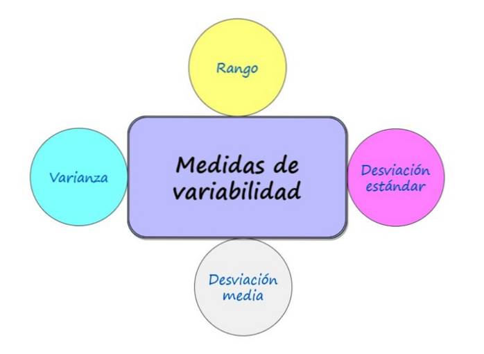
The measures of variability, Also called measures of dispersion, they are statistical indicators that indicate how close or far the data is from its arithmetic mean. If the data are close to the mean, the distribution is concentrated, and if they are far away, then it is a sparse distribution.

There are many measures of variability, among the best known are:

• Rank
• Mean deviation
• Variance
• Standard deviation

These measures complement the measures of central tendency and are necessary to understand the distribution of the data obtained and extract from them as much information as possible..

Rank

Range or span measures the breadth of a data set. To determine its value, find the difference between the data with the highest value x_max and the one with the lowest value x_min:

R = x_max - x_min

If the data is not loose but grouped by interval, then the range is calculated by the difference between the upper limit of the last interval and the lower limit of the first interval.

When the range is a small value it means that all the data are fairly close to each other, but a large range indicates that there is a lot of variability. It is evident that, apart from the upper limit and the lower limit of the data, the range does not take into account the values ​​between them, so it is not recommended to use it when the number of data is large.

However, it is an immediate measure to calculate and has the same units of the data, so it is easy to interpret.

Range example

Below is the list with the number of goals scored during the weekend, in the soccer leagues of nine countries:

40, 32, 35, 36, 37, 31, 37, 29, 39

This is an ungrouped data set. To find the range, we proceed to order them from lowest to highest:

29, 31, 32, 35, 36, 37, 37, 39, 40

The data with the highest value is 40 goals and the one with the lowest value is 29 goals, therefore the range is:

R = 40−29 = 11 goals.

It can be considered that the range is small compared to the minimum value data, which is 29 goals, so it can be assumed that the data do not have great variability.

Mean deviation

This measure of variability is calculated through the average of the absolute values ​​of the deviations with respect to the mean.. Denoting the mean deviation as D_M, For non-grouped data, the mean deviation is calculated using the following formula:

Where n is the number of data available, x_i represents each data and x̄ is the average, which is determined by adding all the data and dividing by n:

The mean deviation allows to know, on average, in how many units the data deviates from the arithmetic mean and has the advantage of having the same units as the data with which we are working.

Example of mean deviation

Based on the data from the range example, the number of goals scored is:

40, 32, 35, 36, 37, 31, 37, 29, 39

If you want to find the mean deviation D_M From these data, it is necessary to first calculate the arithmetic mean x̄:

And now that the value of x̄ is known, we proceed to find the mean deviation D_M:

= 2.99 ≈ 3 goals

Therefore, it can be stated that, on average, the data is approximately 3 goals away from the average, which is 35 goals, and as noted, it is a much more precise measure than the range.

Variance

The mean deviation is a much finer measure of variability than the range, but since it is calculated through the absolute value of the differences between each data and the mean, it does not offer greater versatility from an algebraic point of view..

For this reason, the variance is preferred, which corresponds to the average of the quadratic difference of each data with the mean and is calculated using the formula:

In this expression, s^two denotes the variance, and as always x_i represents each of the data, x̄ is the mean and n is the total data.

When working with a sample instead of the population, it is preferred to calculate the variance like this:

In any case, variance is characterized by always being a positive quantity, but since it is the average of the quadratic differences, it is important to note that it does not have the same units as those of the data..

Variance example

To calculate the variance of the data in the examples of range and mean deviation, we proceed to substitute the corresponding values ​​and perform the indicated summation. In this case, we choose to divide by n-1:

= 13.86

Standard deviation

The variance does not have the same unit as that of the variable under study, for example, if the data comes in meters, the variance results in square meters. Or in the goals example it would be in goals squared, which makes no sense.

Therefore, the standard deviation is defined, also called typical deviation, as the square root of the variance:

s = √s^two

In this way, a measure of variability of the data is obtained in the same units as these, and the lower the value of s, the more grouped the data are around the mean..

Both the variance and the standard deviation are the measures of variability to choose when the arithmetic mean is the measure of central tendency that best describes the behavior of the data..

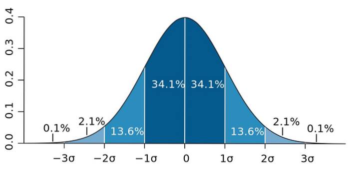
And it is that the standard deviation has an important property, known as Chebyshev's theorem: at least 75% of the observations are in the interval defined by x̄ ± 2s. In other words, 75% of the data is at most 2s away from the mean..

Likewise, at least 89% of the values ​​are at a distance of 3s from the mean, a percentage that can be expanded, as long as there is a lot of data available and they follow a normal distribution..

Figure 2.- If the data follow a normal distribution, 95.4 of them are within two standard deviations on both sides of the mean. Source: Wikimedia Commons.

Standard deviation example

The standard deviation of the data presented in the previous examples is:

s = √s^two = √13.86 = 3.7 ≈ 4 goals