The axial load It is the force that is directed parallel to the axis of symmetry of an element that makes up a structure. The axial force or load can be tension or compression. If the line of action of the axial force coincides with the axis of symmetry that passes through the centroid of the element considered then it is said to be a concentric axial load or force.
On the contrary, if it is an axial force or load parallel to the axis of symmetry, but whose line of action is not on the axis itself, it is an eccentric axial force.
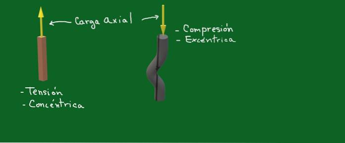
In figure 1 the yellow arrows represent axial forces or loads. In one case it is a concentric tension force and in the other we are dealing with an eccentric compression force.
The unit of measurement for axial load in the SI international system is the Newton (N). But other units of force such as kilogram-force (kg-f) and pound-force (lb-f) are also frequently used..
Article index
To calculate the value of the axial load in the elements of a structure, the following steps must be followed:
- Make the force diagram on each element.
- Apply the equations that guarantee translational equilibrium, that is, that the sum of all forces is zero.
- Consider the equation of torques or moments so that rotational equilibrium is satisfied. In this case the sum of all torques must be zero.
- Calculate the forces, as well as identify the axial forces or loads in each of the elements.
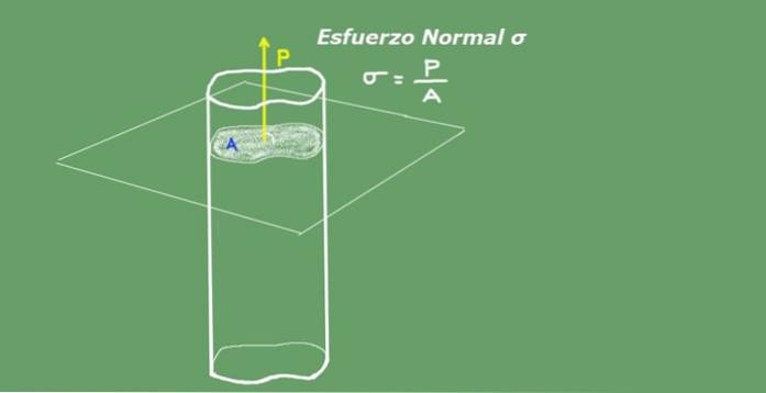
Average normal stress is defined as the ratio of axial load divided by cross-sectional area. The units of normal effort in the International System S.I. they are Newton over square meter (N / m²) or Pascal (Pa). The following figure 2 illustrates the concept of normal stress for clarity..
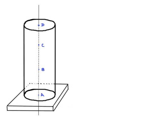
Consider a cylindrical concrete column of height h and radius r. Assume that the density of concrete is ρ. The column does not support any additional load other than its own weight and is supported on a rectangular base.
- Find the value of the axial load at points A, B, C and D, which are in the following positions: A at the base of the column, B a ⅓ of height h, C a ⅔ of height h and by last D at the top of the column.
- Also determine the average normal stress at each of these positions. Take the following numerical values: h = 3m, r = 20cm and ρ = 2250 kg / m³
The total weight W of the column is the product of its density times the volume multiplied by the acceleration of gravity:
W = ρ ∙ h ∙ π ∙ r² ∙ g = 8313 N
At point A the column must support its full weight, so the axial load at this point is compression is equal to the weight of the column:
PA = W = 8313 N
Only ⅔ of the column will be on point B, so the axial load at that point will be compression and its value ⅔ the weight of the column:
PB = ⅔ W = 5542 N
Above position C there is only ⅓ of column, so its axial compression load will be ⅓ of its own weight:
PC = ⅓ W = 2771 N
Finally, there is no load on point D, which is the upper end of the column, so the axial force at that point is zero..
PD = 0 N
To determine the normal stress in each of the positions, it will be necessary to calculate the cross section of area A, which is given by:
A = π ∙ r² = 0.126m²
In this way, the normal stress in each of the positions will be the quotient between the axial force at each of the points divided by the cross-sectional area already calculated, which in this exercise is the same for all the points because it is a column. cylindrical.
σ = P / A; σA = 66.15 kPa; σB = 44.10 kPa; σC = 22.05 kPa; σD = 0.00 kPa
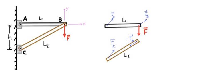
The figure shows a structure made up of two bars that we will call AB and CB. Bar AB is supported at end A by a pin and at the other end connected to the other bar by another pin B.
Similarly, the bar CB is supported at the end C by means of a pin and at the end B with the pin B that joins it to the other bar. A vertical force or load F is applied to pin B as shown in the following figure:
Assume the weight of the bars to be negligible, since the force F = 500 kg-f is much greater than the weight of the structure. The separation between supports A and C is h = 1.5m and the length of the bar AB is L1 = 2 m. Determine the axial load on each of the bars, indicating whether it is compression or tension axial load.
The figure shows, by means of a free-body diagram, the forces acting on each of the elements of the structure. The Cartesian coordinate system with which the force equilibrium equations will be established is also indicated..
Torques or moments will be calculated at point B and will be considered positive if they point away from the screen (Z axis). The balance of forces and torques for each bar is:
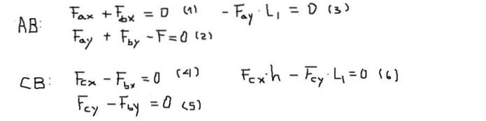
Next, the components of the forces of each of the equations are solved in the following order:
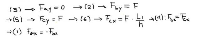
Finally, the resulting forces at the ends of each bar are calculated:
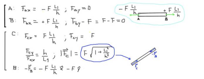
F ∙ (L1 / h) = 500 kg-f ∙ (2.0m / 1.5m) = 666.6 kg-f = 6533.3 N
Bar CB is in compression due to the two forces acting at its ends that are parallel to the bar and are pointing toward its center. The magnitude of the axial compression force in the bar CB is:
F ∙ (1 + L1² / h²) 1/2 = 500 kg-f ∙ (1 + (2 / 1.5) ²) 1/2 = 833.3 kg-f = 8166.6 N


Yet No Comments